The production costs of an enterprise can be divided into two categories: variable and fixed costs. Variable costs depend on changes in the volume of production, while fixed costs remain fixed. Understanding the principle of classifying costs into fixed and variable is the first step to managing costs and improving production efficiency. Knowing how to calculate variable costs can help you lower your unit cost, making your business more profitable.

Steps

Calculation of variable costs

Classify costs as fixed and variable. Fixed costs are those costs that remain unchanged when the volume of production changes. For example, this can include rent and salaries of management personnel. Whether you produce 1 unit per month or 10,000 units, these costs will remain about the same. Variable costs change with changes in the volume of production. For example, they include the cost of raw materials, packaging materials, shipping costs and wages production workers. How more products you produce, the higher will be variable costs.

Add together all variable costs for the time period under consideration. Having identified all variable costs, calculate their total value for the analyzed period of time. For example, your manufacturing operations are quite simple and include only three types of variable costs: raw materials, packaging and shipping costs, and workers' wages. The sum of all these costs will be the total variable costs.

Divide the total variable costs by the volume of production. If you divide the total amount of variable costs by the volume of production for the analyzed period of time, you will find out the amount of variable costs per unit of output. The calculation can be presented as follows: v = V Q (\displaystyle v=(\frac (V)(Q))), where v is the variable cost per unit, V is the total variable cost, and Q is the output. For example, if in the above example the annual production is 500,000 units, then the variable cost per unit would be: 1550000 500000 (\displaystyle (\frac (1550000)(500000))), or 3 , 10 (\displaystyle 3,10) ruble.

Application of the minimax calculation method

1. Find the combined costs. Sometimes some costs cannot be clearly attributed to variable or fixed costs. Such costs may vary depending on the volume of production, but also be present when production is worth or there are no sales. These costs are called combined costs. They can be broken down into fixed and variable components to more accurately determine the amount of fixed and variable costs.

   Estimate costs according to the level of production activity. To break down the combined costs into fixed and variable components, you can use the minimax method. This method evaluates the combined costs for the months with the highest and lowest output, and then compares them to identify the variable cost component. To start the calculation, you must first determine the months with the highest and lowest volume of manufacturing activity (production volume). Record, for each month under consideration, the production activity as some measurable indicator (for example, in terms of machine hours spent) and the corresponding amount of combined costs.

   • Let's say that your company uses a waterjet cutting machine for cutting metal parts in production. For this reason, your company has variable water costs for production, which depend on its volume. However, you also have fixed water costs associated with running your business (drinking, utilities, and so on). In general, the costs of water in your company are combined.
   • Let's assume that in the month with the highest production, your water bill was 9,000 rubles, and at the same time you spent 60,000 machine hours on production. And in the month with the lowest production volume, the water bill was 8,000 rubles, while 50,000 machine hours were spent.

2. Calculate the variable cost per unit of output (VCR). Find the difference between the two values ​​of both indicators (costs and production) and determine the value of variable costs per unit of production. It is calculated as follows: V C R = C − c P − p (\displaystyle VCR=(\frac (C-c)(P-p))), where C and c are the costs for the months with high and low levels of production, and P and p are the corresponding levels of production activity.

   Determine the total variable costs. The value calculated above can be used to determine the variable part of the combined costs. Multiply the variable cost per unit of output by the corresponding level of production activity. In this example, the calculation would be: 0 , 10 × 50000 (\displaystyle 0.10\times 50000), or 5000 (\displaystyle 5000) rubles per month with the lowest production volume, and 0 , 10 × 60000 (\displaystyle 0.10\times 60000), or 6000 (\displaystyle 6000) rubles per month with the highest production volume. This will give you the total variable cost of water in each of the months in question. Then their value can be subtracted from the total value of the combined costs and get the amount of fixed costs for water, which in both cases will be 3,000 rubles.

Using variable cost information in practice

Evaluate trends in variable costs. In most cases, an increase in production will make each additional unit produced more profitable. This is because fixed costs are spread over more units of output. For example, if a business that produced 500,000 units spent 50,000 rubles on rent, these costs in the cost of each unit of production amounted to 0.10 rubles. If the volume of production doubles, then the rental cost per unit of production will already be 0.05 rubles, which will allow you to get more profit from the sale of each unit of goods. That is, as sales revenue increases, the cost of production also increases, but at a slower pace (ideally, in the cost of a unit of production, variable costs per unit should remain unchanged, and a component of fixed costs per unit should fall).

Use the percentage of variable costs in cost to assess risk. If we calculate the percentage of variable costs in the cost of a unit of production, then we can determine the proportional ratio of variable and fixed costs. The calculation is made by dividing the value of variable costs per unit of production by the unit cost of production according to the formula: v v + f (\displaystyle (\frac (v)(v+f))), where v and f are variable and fixed costs per unit of output, respectively. For example, if the fixed costs per unit of production are 0.10 rubles, and the variable costs are 0.40 rubles (for a total cost of 0.50 rubles), then 80% of the cost is variable costs ( 0 , 40 / 0 , 50 = 0 , 8 (\displaystyle 0.40/0.50=0.8)). As an outside investor in the company, you can use this information to assess the potential risk to the company's profitability.

Spend comparative analysis with companies in the same industry. First, calculate the variable costs per unit of output for your company. Then collect data on the value of this indicator from companies in the same industry. This will give you a starting point for evaluating the performance of your company. Higher variable costs per unit of output may indicate that a company is less efficient than others; while a lower value of this indicator can be considered a competitive advantage.

• The value of variable costs per unit of output above the industry average indicates that the company spends more money and resources (labor, materials, utilities) on the production of products than its competitors. This may indicate its low efficiency or the use of too expensive resources in production. In any case, it will not be as profitable as its competitors unless it cuts its costs or increases its prices.
• On the other hand, a company that is able to produce the same goods at a lower cost sells competitive advantage in getting more profit from the established market price.
• This competitive advantage may be based on the use of cheaper materials, cheap labor, or more efficient manufacturing facilities.
• For example, a company that purchases cotton at a lower price than other competitors can produce shirts at lower variable costs and charge lower prices for products.
• Public companies publish their statements on their websites, as well as on the websites of exchanges where their securities are traded. Information about their variable costs can be obtained by analyzing the "Statements of Financial Performance" of these companies.

1. Conduct a break-even analysis. Variable costs (if known) combined with fixed costs can be used to calculate the break-even point for a new manufacturing project. The analyst is able to draw a graph of the dependence of fixed and variable costs on production volumes. With it, he will be able to determine the most profitable level of production.

2.3.1. Production costs in a market economy.

production costs - It is the monetary cost of acquiring the factors of production used. Most cost effective method production is considered to be the one at which production costs are minimized. Production costs are measured in terms of costs incurred.

production costs - costs that are directly related to the production of goods.

Distribution costs - costs associated with the sale of manufactured products.

The economic essence of costs is based on the problem of limited resources and alternative use, i.e. the use of resources in this production excludes the possibility of using it for another purpose.

The task of economists is to choose the most optimal variant of the use of factors of production and minimize costs.

Internal (implicit) costs - this is the cash income that the company donates, independently using its own resources, i.e. These are the returns that could be received by the firm for its own use of resources under the best of possible ways their applications. Opportunity cost is the amount of money needed to divert a particular resource away from the production of good B and use it to produce good A.

Thus, the costs in monetary form, which the company has carried out in favor of suppliers (labor, services, fuel, raw materials) is called external (explicit) costs.

The division of costs into explicit and implicit there are two approaches to understanding the nature of costs.

1. Accounting approach: production costs should include all real, actual costs in cash (wages, rent, opportunity costs, raw materials, fuel, depreciation, social contributions).

2. Economic approach: production costs should include not only actual costs in cash, but also unpaid costs; related to the missed opportunity for the most optimal use of these resources.

short term(SR) - the length of time during which some factors of production are constant, while others are variable.

Constant factors - the total size of buildings, structures, the number of machines and equipment, the number of firms that operate in the industry. Therefore, the possibility of free access of firms in the industry in the short run is limited. Variables - raw materials, the number of workers.

Long term(LR) is the length of time during which all factors of production are variable. Those. during this period, you can change the size of buildings, equipment, the number of firms. In this period, the firm can change all production parameters.

Cost classification

fixed costs (FC) - costs, the value of which in the short term does not change with an increase or decrease in production volume, i.e. they do not depend on the volume of output.

Example: building rent, equipment maintenance, administration salary.

S is the cost.

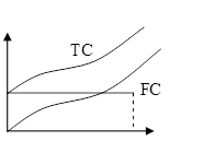
The fixed cost graph is a straight line parallel to the x-axis.

Average fixed costs (A F C) – fixed costs per unit of output and is determined by the formula: A.F.C. = FC/ Q

As Q increases, they decrease. This is called overhead allocation. They serve as an incentive for the firm to increase production.

The graph of average fixed costs is a curve that has a decreasing character, because as the volume of production increases, the total revenue grows, then the average fixed costs are an ever smaller amount that falls on a unit of products.

variable costs (VC) - costs, the value of which varies depending on the increase or decrease in the volume of production, i.e. they depend on the volume of output.

Example: the cost of raw materials, electricity, auxiliary materials, wages (workers). The bulk of the costs associated with the use of capital.

The graph is a curve proportional to the volume of output, which has an increasing character. But its nature can change. In the initial period, variable costs grow at a higher rate than the output. As the optimal size of production (Q 1) is reached, there is a relative saving of VC.

Average variable costs (AVC) – the amount of variable costs per unit of output. They are determined by the following formula: by dividing VC by the volume of output: AVC = VC/Q. First, the curve falls, then it is horizontal and sharply increases.

A graph is a curve that does not start from the origin. General character curve - increasing. Technologically optimal output size is reached when AVCs become minimal (so Q - 1).

Total Costs (TC or C) - a set of fixed and variable costs of the firm, in connection with the production of products in the short run. They are determined by the formula: TC = FC + VC

Another formula (function of volume production products): TC = f(Q).

Depreciation and amortization

Wear is the gradual loss of value by capital resources.

Physical deterioration - loss of consumer qualities by means of labor, i.e. technical and production properties.

The decrease in the value of capital goods may not be associated with the loss of their consumer qualities, then they talk about obsolescence. It is due to an increase in the efficiency of production of capital goods, i.e. the emergence of similar, but cheaper new means of labor, performing similar functions, but more advanced.

Obsolescence is a consequence of scientific and technological progress, but for the company it turns into an increase in costs. Obsolescence refers to changes in fixed costs. Physical wear and tear - to variable costs. Capital goods last more than one year. Their value is transferred to finished products gradually as it wears out - this is called depreciation. Part of the proceeds for depreciation is formed in the depreciation fund.

Depreciation deductions:

Reflect the assessment of the amount of depreciation of capital resources, i.e. are one of the cost items;

Serves as a source of reproduction of capital goods.

The state legislates depreciation rates, i.e. the percentage of the value of capital goods by which they are considered depreciated in a year. It shows how many years the cost of fixed assets should be reimbursed.

Average total cost (ATC) – the sum of the total costs per unit of production:

ATC = TC/Q = (FC + VC)/Q = (FC/Q) + (VC/Q)

The curve is V-shaped. The output corresponding to the minimum average total cost is called the technological optimism point.

Marginal Cost (MC) – the increase in total costs caused by an increase in production by the next unit of output.

Determined by the following formula: MC = ∆TC/ ∆Q.

It can be seen that fixed costs do not affect the value of MC. And MC depends on the increment in VC associated with an increase or decrease in output (Q).

Marginal cost measures how much it will cost a firm to increase output per unit. They decisively influence the choice of the volume of production by the firm, since. this is exactly the indicator that the firm can influence.

The graph is similar to AVC. The MC curve intersects the ATC curve at the point corresponding to the minimum total cost.

In the short run, the company's costs are both fixed and variable. This follows from the fact that production capacity firms remain unchanged and the dynamics of indicators is determined by the growth in equipment utilization.

Based on this graph, you can build a new graph. Which allows you to visualize the capabilities of the company, maximize profits and view the boundaries of the existence of the company in general.

For the decision of the company, the most important characteristic is the average values, the average fixed costs fall as the volume of production increases.

Therefore, the dependence of variable costs on the function of production growth is considered.

At stage I, average variable costs decrease, and then begin to grow under the influence of economies of scale. For this period, it is necessary to determine the break-even point of production (TB).

TB is the level of physical volume of sales over the estimated period of time at which the proceeds from the sale of products coincide with production costs.

Point A - TB, where revenue (TR) = TS

Restrictions that must be observed when calculating TB

1. The volume of production is equal to the volume of sales.

2. Fixed costs are the same for any volume of production.

3. Variable costs change in proportion to the volume of production.

4. The price does not change during the period for which the TB is determined.

5. The price of a unit of production and the cost of a unit of resources remains constant.

Law of diminishing returns is not absolute, but relative, and it operates only in the short term, when at least one of the factors of production remains unchanged.

Law: with an increase in the use of one factor of production, while the rest remain unchanged, sooner or later a point is reached, starting from which the additional use of variable factors leads to a decrease in the increase in production.

The action of this law assumes the immutability of the state of technically and technologically production. And so technological progress can change the scope of this law.

The long run is characterized by the fact that the firm is able to change all the factors of production used. In this period variable nature of all applied factors of production allows the firm to use the most optimal options for their combination. This will be reflected in the magnitude and dynamics of average costs (costs per unit of output). If the company decided to increase the volume of production, but at the initial stage (ATS) will first decrease, and then, when more and more new capacities are involved in production, they will begin to increase.

The graph of long-term total costs shows seven different options (1 - 7) for the behavior of ATS in the short term, since The long run is the sum of the short runs.

The long run cost curve consists of options called growth steps. In each stage (I - III) the firm operates in the short run. The dynamics of the long-run cost curve can be explained using scale effect. Change by the firm of the parameters of its activities, i.e. the transition from one version of the size of the enterprise to another is called change in the scale of production.

I - on this time interval, long-term costs decrease with an increase in the volume of output, i.e. there is economies of scale - a positive scale effect (from 0 to Q 1).

II - (this is from Q 1 to Q 2), at this time interval of production, the long-term ATS does not react in any way to an increase in production volume, i.e. remains unchanged. And the firm will have constant returns to scale (constant returns to scale).

III - long-term ATS with an increase in output grow and there is a loss from the increase in the scale of production or negative scale effect(from Q 2 to Q 3).

3. IN general view profit is defined as the difference between total revenue and total costs for a certain period of time:

SP = TR –TS

TR ( total revenue) - the amount of cash receipts by the company from the sale of a certain amount of goods:

TR = P* Q

AR(average revenue) is the amount of cash receipts per unit of products sold.

Average revenue is equal to the market price:

AR = TR/ Q = PQ/ Q = P

MR(marginal revenue) is the increase in revenue that arises from the sale of the next unit of production. Under perfect competition, it is equal to the market price:

MR = ∆ TR/∆ Q = ∆(PQ) /∆ Q =∆ P

In connection with the classification of costs into external (explicit) and internal (implicit) different concepts of profit are assumed.

Explicit costs (external) determined by the amount of expenses of the enterprise to pay for the purchased factors of production from the outside.

Implicit costs (internal) determined by the cost of resources owned by the enterprise.

If we subtract external costs from total revenue, we get accounting profit - takes into account external costs, but does not take into account internal ones.

If we subtract internal costs from accounting profit, we get economic profit.

Unlike accounting profit, economic profit takes into account both external and internal costs.

Normal profit appears in the case when the total revenue of an enterprise or firm is equal to the total costs, calculated as alternative. The minimum level of profitability is when it is profitable for an entrepreneur to do business. "0" - zero economic profit.

economic profit(net) - its presence means that resources are used more efficiently at this enterprise.

Accounting profit exceeds the economic one by the amount of implicit costs. Economic profit serves as a criterion for the success of the enterprise.

Its presence or absence is an incentive to attract additional resources or transfer them to other areas of use.

The purpose of the firm is to maximize profit, which is the difference between total revenue and total costs. Since both costs and income are a function of the volume of production, the main problem for the firm is to determine the optimal (best) volume of production. The firm will maximize profit at the level of output at which the difference between total revenue and total cost is greatest, or at the level at which marginal revenue equals marginal cost. If the firm's losses are less than its fixed costs, then the firm should continue to operate (in the short run), if the losses are greater than its fixed costs, then the firm should stop production.

Previous

marginal cost() is the cost of producing an additional unit of output.

MC = ∆TC / ∆Q

Marginal cost reflects the change in cost that an increase or decrease in production by one unit would entail.

Comparison of Average and Marginal Costs of Production − important information for the management of the firm, which determines the optimal size of production. At point B, the supply price coincides with average and marginal cost. This point represents the equilibrium of the firm.

When moving from point B to the right, an increase in production leads to a decrease in profit, because additional costs increase for each unit of goods. Going beyond point B leads to the instability of the company's finances and in the end its behavior will be determined by the flight from market structures.

marginal revenue

In modern market economy the calculation of production efficiency involves comparing marginal revenue and marginal cost.

There are two ways to determine the best production volumes. Both are based on a comparison of marginal revenue and marginal cost.

1st method: accounting and analytical

How to determine the marginal cost of producing a third good? To answer this question, we take column 4 with the designation of gross costs. With the transition from the second product to the production of the third, the costs increased (355-340=15). This is the marginal cost associated with the production of the third good.

The most profitable volume of production is at the 6th position, after it the marginal cost already exceeds the marginal revenue, which is clearly unfavorable for the firm.

2nd way: graphic

Based on a comparison of marginal cost and marginal revenue.

The benchmarks for the firm are as follows:

• If marginal revenue is higher than marginal cost, production can be expanded.
• If marginal revenue is less than marginal cost, production is unprofitable and must be curtailed.

The equilibrium point of the firm and maximum profit is reached in the case of equality of marginal revenue and marginal cost.

The equilibrium of a firm under perfect competition, when it chooses the optimal output, implies the following equality:

P = MS + MR

where: P is the price of the good, MC is the marginal cost, MR is the marginal revenue.

Average cost

In order to more clearly define the possible volumes of production at which it protects itself from excessive growth, the dynamics of average costs is examined.

If the gross costs are attributed to the quantity of output, we get average cost(curve ).

This type of average cost curve is determined by the following circumstances: Average costs are:

Average fixed costs are fixed costs per unit of output.

Average variable costs are the variable costs per unit of output.

Unlike average fixed costs, average variable costs can either decrease or increase as output increases, which is explained by the dependence of total variable costs on output. Average variable costs!!AVC?? reach their minimum at a volume that provides maximum value middle product .

Let's prove this position:

Average variable cost (by definition), but

and the output volume.

Thus,

If , then , , which was to be proved.

Average total costs (total) costs - show the total cost per unit of output.

The company's costs in the long run

In the long run all resources of the firm are variable. The firm can hire new equipment, rent new workshops, change the composition management personnel, use new technology production.

The lack of permanent resources in the long run leads to the fact that there is no difference between constant and variable costs . The analysis of the long-term activity of the company is carried out through consideration of the dynamics long run average cost (LATC). And the main goal of the company in the field of costs can be considered the organization of production of the "required scale", providing a given volume of production with lowest average cost.

Long run average cost

To construct long-run average costs, suppose that a firm can organize production of three sizes: small, medium and large, each of which has its own short-run average cost curve (respectively SATC1, SATC2, SATC3), as shown in Fig. 1.

Rice. 1. Long run average cost curve

The choice of one project or another will depend on estimates of projected market demand on the company's products and on what capacities are needed to provide it.

If the forecasted demand corresponds to Q1, then the firm will prefer the creation of small production, since its average costs in this case will be much lower than in more large enterprises. As seen in fig. 1,

ATC1(Q1)2(Q1),

and correspondingly

ATC1(Q1)3(Q1).

If demand is expected to be Q2, then project 2 (medium enterprise) will be the most preferable, providing lower costs, or

ATC2(Q2)1(Q2),

ATC2(Q2)3(Q3).

Similarly, when assessing demand in Q3, the firm will choose a large enterprise.

Combining the segments of the three short-run cost curves that provide the optimal production size for each output, shows us the firm's long-run average cost curve. On fig. 1 is represented by a solid line.

Long run average cost curve shows the minimum cost per unit of output produced at each possible volume of production.

If the number of possible sizes ( Q1, Q2,...Qn) approaches infinity (n → ∞), then the long-run average cost curve becomes flatter, as shown in Fig. 2.

Rice. 2. Curve of long-run average costs with an unlimited number of possible sizes of the enterprise

In this case, all points on the LATC curve are the least average cost at a given output, provided the firm has enough time to change all the required inputs.

Minimum efficient enterprise size

Analysis of long-term average costs reveals optimal enterprise size (Q*), i.e. the amount of production that ensures the minimum cost per unit of output in a given sphere of production. If the LATC curve has a horizontal section, as is the case in Fig. 2, enterprises of several sizes can be considered equally efficient.

The smallest firm size that allows a firm to minimize its long-run average cost is called the minimum efficient size of the enterprise.

Depending on the specifics of production and technological features the minimum effective size can vary widely. Thus, it is estimated that in the production of footwear this indicator is 0.2% of the total output of the industry, in the production of cigarettes - 6.6%, and in the production of cars - 11%.

If the minimum efficient size of one enterprise provides almost 100% of the market needs for a given product, then the firm that owns such an enterprise turns out to be natural monopoly(more details in the topic "Pure monopoly").

Comparison of short and long run average cost curves

Average costs in both the long and short run are the firm's costs per unit of output and are calculated using the same formula:

ATC=TC/Q.

However, there are also fundamental differences:

if in the short run average total costs break down into average fixed and average variable costs

SATC=AVC+AFC,

then in the long run this division does not take place, since all costs are variable;

in the short term U-shaped curves ATC And AVC determined law of diminishing returns variable resource; in the long run, when all resources are variable, the shape of the curves LATC is determined;

for a rationally operating firm choosing the optimal size of the enterprise, long-run average costs are always less than or equal (in other words, no more) than short-run average costs,

SATC≤ LATC (Q*)

Where Q*- optimal production size.

Graphically, this means that the long-run cost curve bends around the short-run cost curves from below.

Scale effect of production

• Main article:

Allows you to calculate the minimum price of goods / services, determine the optimal sales volume and calculate the value of the company's expenses. There are various methods for calculating the types of costs, the main ones are given below.

Production Costs - Calculation Formulas

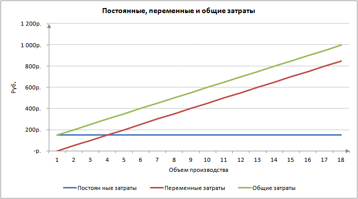
The calculation of production costs is easily performed based on budget documentation. If such forms are not compiled in the organization, data from the reporting period will be required. accounting. It should be borne in mind that all costs are divided into fixed (the value is unchanged over the period) and variable (the value varies depending on the volume of production).

Total production costs - formula:

Total costs = Fixed costs + Variable costs.

This method of calculation allows you to find out the total costs for the entire production. Detailing is carried out by departments of the enterprise, workshops, product groups, types of products, etc. An analysis of indicators in dynamics will help predict the value of production or sales, expected profit / loss, the need to increase capacity, and the inevitability of reducing expenditures.

Average production costs - formula:

Average costs \u003d Total costs / Volume of manufactured products / services performed.

This indicator is also called the total cost of the product/service. Allows you to determine the level minimum price, calculate the efficiency of investing resources for each unit of production, compare mandatory costs with prices.

Marginal cost of production - formula:

Marginal Costs = Change in Total Costs / Change in Output.

The indicator of the so-called additional costs allows you to determine the increase in the cost of issuing an additional volume of GP in the most profitable way. At the same time, the value of fixed costs remains unchanged, variable costs increase.

Note! In accounting, the expenses of the enterprise are reflected in the expense accounts - 20, 23, 26, 25, 29, 21, 28. To determine the costs for the required period, you should sum up the debit turnovers on the accounts involved. Exceptions are internal turnovers and balances at refineries.

How to calculate production costs - an example

GP output volume, pcs.	Total costs, rub.	Average costs, rub.	Fixed costs, rub.	Variable costs, rub.

From the above example, it can be seen that the organization incurs fixed costs in the amount of 1200 rubles. in any case - in the presence or absence of production of goods. Variable costs for 1 pc. initially amount to 150 rubles, but the costs are reduced with the growth of production. This can be seen from the analysis of the second indicator - Average costs, the decrease of which occurred from 1350 rubles. up to 117 rubles. per 1 unit finished product. Marginal cost calculation can be determined by dividing the increase in variable costs by 1 unit of product or by 5, 50, 100, etc.

Let's talk about the fixed costs of the enterprise: what is the economic meaning of this indicator, how to use and analyze it.

Fixed costs. Definition

fixed costs(EnglishFixedcost,FC,TFC ortotalfixedcost) is a class of enterprise costs that are not related (do not depend) on the volume of production and sales. At each moment of time they are constant, regardless of the nature of the activity. Fixed costs combined with variables, which are the opposite of fixed costs, constitute the total costs of the enterprise.

Formula for calculating fixed costs/costs

The table below lists possible fixed costs. In order to better understand fixed costs, we compare them with each other.

fixed costs= Cost of wages + Rent of premises + Depreciation + Property taxes + Advertising;

Variable costs = Costs for raw materials + Materials + Electricity + Fuel + Bonus part of salary;

General costs= Fixed costs + Variable costs.

It should be noted that fixed costs are not always fixed, because an enterprise, with the development of its capacities, can increase production areas, the number of personnel, etc. As a result, fixed costs will also change, which is why management accounting theorists call them ( semi-fixed costs). Similarly, for variable costs - conditionally variable costs.

An example of calculating fixed costs in an enterprise inexcel

We will show clearly the differences between fixed and variable costs. To do this, in Excel, fill in the columns with "production volume", "fixed costs", "variable costs" and "total costs".

Below is a graph comparing these costs with each other. As we can see, with an increase in production, the constants do not change with time, but the variables increase.

Fixed costs do not change only in the short run. In the long run, any costs become variable, often due to the impact of external economic factors.

Two Methods for Calculating Costs in an Enterprise

In the production of products, all costs can be divided into two groups according to two methods:

• fixed and variable costs;
• indirect and direct costs.

It should be remembered that the costs of the enterprise are the same, only their analysis can be carried out using different methods. In practice, fixed costs are strongly intersected with such a concept as indirect costs or overhead costs. As a rule, the first method of cost analysis is used in management accounting, and the second in accounting.

Fixed costs and the break-even point of the enterprise

Variable costs are part of the break-even point model. As we determined earlier, fixed costs do not depend on the volume of production / sales, and with an increase in output, the enterprise will reach a state where the profit from the sold products will cover variable and fixed costs. This state is called the break-even point or critical point, when the company becomes self-sufficient. This point is calculated in order to predict and analyze the following indicators:

• at what critical volume of production and sales the enterprise will be competitive and profitable;
• how much sales need to be made in order to create a zone of financial security for the enterprise;

Marginal profit (income) at the break-even point coincides with the fixed costs of the enterprise. Domestic economists often use the term gross income instead of marginal profit. The more contribution margin covers fixed costs, the higher the profitability of the enterprise. You can study the break-even point in more detail in the article ““.

Fixed costs in the balance sheet of the enterprise

Since the concepts of fixed and variable costs of the enterprise refer to management accounting, then there are no lines in the balance sheet with such names. In accounting (and tax accounting), the concepts of indirect and direct costs are used.

In the general case, fixed costs include balance lines:

• Cost of goods sold - 2120;
• Commercial expenses - 2210;
• Management (general) - 2220.

The figure below shows the balance sheet of OJSC “Surgutneftekhim”, as we can see, fixed costs change every year. The fixed cost model is a purely economic model, and it can be used in the short run, when revenue and output change linearly and regularly.

Let's take another example - OJSC ALROSA and look at the dynamics of changes in conditionally fixed costs. The figure below shows how costs have changed from 2001 to 2010. It can be seen that the costs were not constant over 10 years. The most stable costs throughout the period were selling expenses. The rest of the costs have changed in one way or another.

Summary

Fixed costs are costs that do not change with the volume of production of the enterprise. This type cost is used in management accounting to calculate the total costs and determine the break-even level of the enterprise. Since the company operates in a constantly changing external environment, then fixed costs in the long run also change and therefore in practice they are often called conditionally fixed costs.